Visualizing molecular orbitals

← Previous | Next →
July 21, 2022 (2022-07-21 23:00:00) by Anders Lervik | Category: chemistry
Tagged: chemistry | jupyter | molecules | orbitals | python

Introduction

In this post, I will calculate molecular orbitals (MOs) and visualize them. Here is an example for butadiene:

Calculating MOs is relatively straightforward with pyscf, and visualizing them can be done (directly in jupyter) with py3Dmol or fortecubeview. fortecubeview is easier to use (it has an interface that allows us to browse through different MOs) while py3Dmol can be customized more, and also supports creating grids to display several models simultaneously.

Both py3Dmol and fortecubeview are based on reading cube files so the code below will write out those. This also means that you can load the cube file(s) in your favorite molecular viewer (for instance, vmd) and customize the visualization.

Note

The pyscf calculation below will use a small basis set to make the computations run faster.

Calculating molecular orbitals

For calculating molecular orbitals, I will run a restricted Hartree Fock calculation with pyscf. I will use the geometry that RDKit generates, and I will not optimize the geometry with pyscf here to save some computational time.

For visualizing the molecular orbitals, I will calculate both the canonical molecular orbitals and the intrinsic bond orbitals (IBO).

I begin by importing RDKit (used for generating coordinates), py3Dmol and fortecubeview (used for visualization), matplotlib and seaborn (used for plotting), pandas and numpy (used for some numerics results), and pyscf (used for the quantum mechanics).

import pathlib

# RDKit imports:
from rdkit import Chem
from rdkit.Chem import (
    AllChem,
    rdCoordGen,
)
from rdkit.Chem.Draw import IPythonConsole

IPythonConsole.ipython_useSVG = True  # Use higher quality images for molecules

# For visualization of molecules and orbitals:
import py3Dmol
import fortecubeview

# pyscf imports:
from pyscf import gto, scf, lo, tools

# For plotting
import matplotlib
from matplotlib import pyplot as plt
import seaborn as sns

%matplotlib inline
sns.set_theme(style="ticks", context="talk", palette="muted")

# For numerics:
import numpy as np
import pandas as pd

pd.options.display.float_format = "{:,.3f}".format

Set up the molecule with RDKit

For this example, I will use ethene - it is a simple molecule and from basic chemistry we expect to see a π-bond.

molecule_name = "ethene"
molecule = Chem.MolFromSmiles("C=C")  # Generate the molecule from smiles
molecule

def get_xyz(molecule, optimize=False):
    """Get xyz-coordinates for the molecule"""
    mol = Chem.Mol(molecule)
    mol = AllChem.AddHs(mol, addCoords=True)
    AllChem.EmbedMolecule(mol)
    if optimize:  # Optimize the molecules with the MM force field:
        AllChem.MMFFOptimizeMolecule(mol)
    xyz = []
    for lines in Chem.MolToXYZBlock(mol).split("\n")[2:]:
        strip = lines.strip()
        if strip:
            xyz.append(strip)
    xyz = "\n".join(xyz)
    return mol, xyz

molecule3d, xyz = get_xyz(molecule)

view = py3Dmol.view(
    data=Chem.MolToMolBlock(molecule3d),
    style={"stick": {}, "sphere": {"scale": 0.3}},
    width=300,
    height=300,
)
view.zoomTo()

You appear to be running in JupyterLab (or JavaScript failed to load for some other reason). You need to install the 3dmol extension:
jupyter labextension install jupyterlab_3dmol

<py3Dmol.view at 0x7f0976544f10>

Run pyscf and calculate molecular orbitals

def run_calculation(xyz, basis="sto-3g"):
    """Calculate the energy (+ additional things like MO coefficients) with pyscf."""
    mol = gto.M(
        atom=xyz,
        basis=basis,
        unit="ANG",
        symmetry=True,
    )
    mol.build()
    mf = scf.RHF(mol).run()
    return mf, mol

mf, mol = run_calculation(xyz, basis="sto-3g")

converged SCF energy = -77.069961819782

To show some results from the calculation (for instance energies and contributions to the molecular orbitals) we can make use of mf.analyze. This is commented out here to reduce the output.

# mf.analyze(verbose=5)

We can access the energy and occupancy of the molecular orbitals via the .mo_energy and .mo_occ attributes:

table = pd.DataFrame({"Energy": mf.mo_energy, "Occupancy": mf.mo_occ})
table

	Energy	Occupancy
0	-11.017	2.000
1	-11.016	2.000
2	-0.986	2.000
3	-0.735	2.000
4	-0.616	2.000
5	-0.519	2.000
6	-0.466	2.000
7	-0.330	2.000
8	0.326	0.000
9	0.652	0.000
10	0.661	0.000
11	0.690	0.000
12	0.968	0.000
13	1.004	0.000

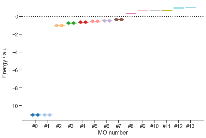
Let us also make a plot of the energy levels:

fig, ax = plt.subplots(constrained_layout=True, figsize=(9, 6))
colors = matplotlib.cm.get_cmap("tab20")(np.linspace(0, 1, len(mf.mo_energy)))

pos = []
for i, (energy, occ) in enumerate(zip(mf.mo_energy, mf.mo_occ)):
    left = 3 * i
    right = 3 * i + 2.5
    length = right - left

    (line,) = ax.plot([left, right], [energy, energy], color=colors[i], lw=3)

    electron_x, electron_y = None, None
    if occ == 2:
        electron_x = [left + 0.25 * length, left + 0.75 * length]
        electron_y = [energy, energy]
    elif occ == 1:
        electron_x, electron_y = [left + 0.5], [energy]
    if electron_x and electron_y:
        ax.scatter(electron_x, electron_y, color=line.get_color())

    pos.append(left + 0.5 * length)

ax.axhline(y=0, ls=":", color="k")
ax.set_xticks(pos)
ax.set_xticklabels([f"#{i}" for i, _ in enumerate(pos)])
ax.set(xlabel="MO number", ylabel="Energy / a.u.")
sns.despine(fig=fig)

OK, so we have the energies and occupancy. But now, we would like to display the orbitals. The canonical ones are available via mf.mo_coeff. For the intrinsic bonding orbitals, we will have to do some additional calculations. This is defined in the method below. In addition, this method will obtain the localized intrinsic valence virtual orbitals (LIVVO):

def get_mo(mf, mol):
    """Get molecular orbitals"""
    orbitals = {"canonical": mf.mo_coeff}

    # Get intrinsic bonding orbitals and localized intrinsic valence virtual orbitals (livvo):
    orbocc = mf.mo_coeff[:, 0 : mol.nelec[0]]
    orbvirt = mf.mo_coeff[:, mol.nelec[0] :]

    ovlpS = mol.intor_symmetric("int1e_ovlp")

    iaos = lo.iao.iao(mol, orbocc)
    iaos = lo.orth.vec_lowdin(iaos, ovlpS)
    ibos = lo.ibo.ibo(mol, orbocc, locmethod="IBO")
    orbitals["ibo"] = ibos

    livvo = lo.vvo.livvo(mol, orbocc, orbvirt)
    orbitals["livvo"] = livvo
    return orbitals

orbitals = get_mo(mf, mol)

 Iterative localization: IB/P4/2x2, 7 iter; Final gradient 9.97e-10
 Iterative localization: IB/P4/2x2, 6 iter; Final gradient 6.31e-09

Visualizing the orbitals with py3Dmol and fortecubeview

For visualizing the molecular orbitals, it is convenient to write them as cube files. These cube files can be visualized in jupyter by py3Dmol or fortecubeview, or in external programs such as VMD.

Here is a short method to write the cube files for some given molecular orbital coefficients:

def write_all_coeffs(
    mol, coeffs, prefix="cmo", dirname=".", margin=5, offset=0
):
    """Write cube files for the given coefficients."""
    path = pathlib.Path(dirname)
    path.mkdir(parents=True, exist_ok=True)

    for i in range(coeffs.shape[1]):
        outfile = f"{prefix}_{i+offset:02d}.cube"
        outfile = path / outfile
        print(f"Writing {outfile}")
        tools.cubegen.orbital(mol, outfile, coeffs[:, i], margin=margin)

To write all the canonical molecular orbitals write_all_coeffs can be used as follows:

# write_all_coeffs(
#    mol,
#    orbitals["canonical"],
#    prefix=f"{molecule_name}_cmo",
#    dirname="cmo",
#    margin=5,
# )

And to write all the IBOs and LIVVOs:

# write_all_coeffs(
#    mol,
#    orbitals["ibo"],
#    prefix=f"{molecule_name}_ibo",
#    dirname="ibo",
#    margin=5,
# )

# write_all_coeffs(
#    mol,
#    orbitals["livvo"],
#    prefix=f"{molecule_name}_livvo",
#    dirname="ibo",
#    margin=5,
#    offset=orbitals["ibo"].shape[1],
# )

For simplicity, I will only write the highest occupied orbital and the lowest unoccupied orbital here:

def find_homo_lumo(mf):
    lumo = float("inf")
    lumo_idx = None
    homo = -float("inf")
    homo_idx = None
    for i, (energy, occ) in enumerate(zip(mf.mo_energy, mf.mo_occ)):
        if occ > 0 and energy > homo:
            homo = energy
            homo_idx = i
        if occ == 0 and energy < lumo:
            lumo = energy
            lumo_idx = i

    return homo, homo_idx, lumo, lumo_idx


_, homo_idx, _, lumo_idx = find_homo_lumo(mf)
print(f"HOMO (index): {homo_idx}")
print(f"LUMO (index): {lumo_idx}")

HOMO (index): 7
LUMO (index): 8

tools.cubegen.orbital(
    mol, "cmo_homo.cube", orbitals["canonical"][:, homo_idx], margin=5
)
tools.cubegen.orbital(
    mol, "cmo_lumo.cube", orbitals["canonical"][:, lumo_idx], margin=5
)
tools.cubegen.orbital(mol, "ibo_homo.cube", orbitals["ibo"][:, -1], margin=5)
tools.cubegen.orbital(
    mol, "livvo_lumo.cube", orbitals["livvo"][:, 0], margin=5
);

To display the molecular orbitals, fortecubeview is really convenient as we can give it a directory, and it will load all the cube files in that directory:

fortecubeview.plot(path=".", sumlevel=0.85)

CubeViewer: listing cube files from the directory .
Reading 4 cube files

<fortecubeview.cube_viewer.CubeViewer at 0x7f096fb8a280>

We can also use py3Dmol. First, we read the cube file we want, and then we pass that to py3Dmol:

data = None
with open("ibo_homo.cube", "r") as infile:
    data = infile.read()

view = py3Dmol.view()
view.addVolumetricData(
    data,
    "cube",
    {
        "isoval": 0.05,
        "smoothness": 5,
        "opacity": 0.8,
        "volformat": "cube",
        "color": "blue",
    },
)
view.addVolumetricData(
    data,
    "cube",
    {
        "isoval": -0.05,
        "smoothness": 5,
        "opacity": 0.8,
        "volformat": "cube",
        "color": "orange",
    },
)
view.addModel(data, "cube")
view.setStyle({"stick": {}})
view.zoomTo()
view.show()

Note

The interactive part is not shown in the output above, since the generated cube files are large. They can be found in the binder notebook:

Summary

With the code above, we can visualize molecular orbitals. The output from the last cell above (the visualization with py3Dmol) looks like this:

and this shows something very similar to the expected π bond. We can also try the code above for other molecules, for instance, benzene (note RDKit might generate a structure where pyscf does not find the correct symmetry). Here are the 5 highest binding molecular orbitals of benzene

and the lowest unoccupied orbital: