Calculating the pH in weak acids#
← Previous | Oldest ↻ August 02, 2022 () by Anders Lervik | Category: chemistry Tagged: chemistry
Introduction#
If you have taken a chemistry course, you have probably calculated the pH in a weak acid. A typical problem is: What is the pH in a solution of the weak acid HA (with concentration C) in water? The solution can then be found by solving,
where \(K_\text{a}\) is the acid dissociation constant, and \(x\) is the (unknown) concentration of hydrogen ions. We assume here that we do not have to take the autoionization of water into consideration, but when is this true? I will check this with some calculations here.
Note
To give you the answer right now: Solve the equation given above. If the pH is 6 or smaller, this is good enough. If the pH is above 6, solve the more complex equations given below.
Calculating the pH in a weak acid#
I consider the dissociation of the weak acid HA:
We have the following equations:
The equilibrium constant for the acid dissociation: \(K_\text{a} = \frac{[\text{H}^+] [\text{A}^-]}{[\text{HA}]}\).
The equilibrium constant for autoionization of water: \(K_\text{w} = [\text{H}^+] [\text{OH}^-]\).
The mass balance (based on element A): \([\text{HA}]_0 = [\text{HA}] + [\text{A}^-]\), where \([\text{HA}]_0\) is the initial concentration of HA.
The electroneutrality: \([\text{H}^+] = [\text{A}^-] + [\text{OH}^-]\).
We can rewrite the electroneutrality as \([\text{A}^-] = [\text{H}^+] - \frac{K_\text{w}}{[\text{H}^+]}\), combine it with the mass balance and the equilibrium constant to get:
which is an equation with one unknown (\([\text{H}^+]\)) we can solve.
We can also recover the usual General Chemistry 101 formula by assuming that \([\text{H}^+]^2 \gg K_\text{w}\):
Solving the approximate equation#
The approximate equation is a quadratic equation, \([\text{H}^+]^2 + [\text{H}^+] K_\text{a} - K_\text{a} [\text{HA}]_0 = 0.\) and we can solve it by:
[1]:
import numpy as np
import warnings
[2]:
@np.vectorize
def calculate_ph_approximate(c_ha_zero, ka):
    """Solve the approximate equation"""
    poly = [1, ka, -ka * c_ha_zero]
    discriminant = poly[1] ** 2 - 4 * poly[0] * poly[2]
    if discriminant < 0:
        raise ValueError("No positive roots!")
    # Calculate the positive root:
    x = (-poly[1] + np.sqrt(discriminant)) / (2 * poly[0])
    return -np.log10(x)
Let us try this for Example 15.9.2 from Principles of modern chemistry (where the pH is calculated to be 6.65):
[3]:
calculate_ph_approximate(0.001, 4.0e-11)
[3]:
array(6.69901343)
The approximate solution is not spot on here, but it is pretty close.
Solving the full equation#
The full equation can be rewritten as a cubic equation:
According to Descartes’ rule this equation will have exactly one positive root. We can also use the base constant:
I will use the first equation and solve for \([\text{H}^+]\), but if there are some issues with the solution, I will use the equation for \([\text{OH}^-]\). To check if there are some issues, I define two simple checks below:
[4]:
def check_solution_acid(c_ha_zero, ka, kw, x, print_warning=False):
    """Do some checks for the solution."""
    c_OH = kw / x
    c_A = x - c_OH
    w = 0
    if c_A < 0:
        if print_warning:
            warnings.warn(f"Unphysical [A-] = {c_A} for {c_ha_zero}, {ka}")
        w += 1
    c_HA = c_ha_zero - c_A
    if c_HA < 0:
        if print_warning:
            warnings.warn(f"Unphysical [HA] = {c_HA} for {c_ha_zero}, {ka}")
        w += 1
    ka_ = x * c_A / c_HA
    if not np.isclose(ka_, ka, atol=1e-6):
        if print_warning:
            warnings.warn(
                f"Solution is inconsistent for {c_ha_zero}, {ka_} != {ka}"
            )
        w += 1
    return w


def check_solution_base(c_ha_zero, ka, kw, x, print_warning=False):
    """Do some checks for the solution."""
    c_H = kw / x
    c_A = c_H - x
    w = 0
    if c_A < 0:
        if print_warning:
            warnings.warn(f"Unphysical [A-] = {c_A} for {c_ha_zero}, {ka}")
        w += 1
    c_HA = c_ha_zero - c_A
    if c_HA < 0:
        if print_warning:
            warnings.warn(f"Unphysical [HA] = {c_HA} for {c_ha_zero}, {ka}")
        w += 1
    kb = kw / ka
    kb_ = x * c_HA / c_A
    if not np.isclose(kb_, kb, atol=1e-6):
        if print_warning:
            warnings.warn(
                f"Solution is inconsistent for {c_ha_zero}, {kb_} != {kb}"
            )
        w += 1
    return w
[5]:
@np.vectorize
def calculate_ph_full(c_ha_zero, ka, kw=1e-14):
    """Solve the full equation"""
    poly_h = [1, ka, -(kw + ka * c_ha_zero), -ka * kw]
    roots_h = np.roots(poly_h)
    # Select the positive solution:
    x_h = roots_h[roots_h > 0][0]
    # Do some checks:
    w = check_solution_acid(c_ha_zero, ka, kw, x_h, print_warning=False)
    if w > 0:  # Fix problems by solving the base equation:
        kb = kw / ka
        poly_oh = [1, (c_ha_zero + kb), -kw, -kb * kw]
        roots_oh = np.roots(poly_oh)
        x_oh = roots_oh[roots_oh > 0][0]
        x_h = kw / x_oh
        check_solution_base(c_ha_zero, ka, kw, x_oh, print_warning=True)
    return -np.log10(x_h)
I will also try this method for Example 15.9.2 from Principles of modern chemistry (where the pH is calculated to be 6.65):
[6]:
calculate_ph_full(0.001, 4.0e-11)
[6]:
array(6.65054607)
Ah, this is a more accurate result! I will run some more comparisons below.
Comparing the solutions#
[7]:
from matplotlib import pyplot as plt
import seaborn as sns
import matplotlib as mpl

%matplotlib inline

mpl.rcParams["ytick.minor.visible"] = True
mpl.rcParams["xtick.minor.visible"] = True
sns.set_theme(style="ticks", context="talk", palette="muted")
[8]:
ka = [1e-2, 1e-4, 1e-8, 1e-10]
concentrations = 10.0 ** np.arange(-12, 3, 1)

fig, axes = plt.subplots(
    constrained_layout=True, ncols=4, figsize=(12, 3), sharex=True, sharey=True
)

for kai, axi in zip(ka, axes):
    ph_approx = calculate_ph_approximate(concentrations, kai)
    ph_full = calculate_ph_full(concentrations, kai)
    axi.scatter(-np.log10(concentrations), ph_approx, label="Approximate")
    axi.scatter(-np.log10(concentrations), ph_full, label="Full solution")
    axi.set(xlabel="pC", title=f"pKa = {-np.log10(kai)}")
axes[0].set(ylabel="pH")
axes[0].legend()
sns.despine(fig=fig)

We do get some errors for low concentrations here. Let us investigate a grid of points:
[9]:
ka = 10.0 ** np.arange(-14, 1, 0.2)
concentrations = 10.0 ** np.arange(-14, 2, 0.2)
ka_grid, conc_grid = np.meshgrid(ka, concentrations)
ph_approx = calculate_ph_approximate(conc_grid, ka_grid)
ph_full = calculate_ph_full(conc_grid, ka_grid)
error_grid = abs(ph_approx - ph_full) / abs(ph_full)
[10]:
fig, ax = plt.subplots(constrained_layout=True, figsize=(10, 8))
im = ax.contourf(
    -np.log10(conc_grid),
    -np.log10(ka_grid),
    error_grid * 100,
    cmap="vlag",
    levels=40,
)

im2 = ax.contour(
    -np.log10(conc_grid),
    -np.log10(ka_grid),
    error_grid * 100,
    levels=[1, 10],
    colors="w",
)

ax.clabel(
    im2, im2.levels, inline=True, fontsize="small", fmt="Error = %.1f %%"
)


ax.set(xlabel="pC", ylabel="pKa")

ax.scatter(-np.log10(0.001), -np.log10(4e-11), color="white")
ax.annotate(
    "Example calculation",
    (-np.log10(0.001), -np.log10(4e-11)),
    xytext=(-100, -75),
    color="white",
    textcoords="offset points",
    arrowprops={"arrowstyle": "->"},
)
fig.colorbar(im, ax=ax, label="Error (%)")
[10]:
<matplotlib.colorbar.Colorbar at 0x7fb8165fef40>
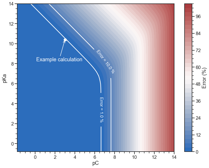
To get an error below 1%:
- If the concentration is lower than \(10^{-6.7} = 2 \times 10^{-7}\) we should not use the approximation.
- If the concentration is higher than \(2 \times 10^{-7}\) , we can use it as long as \(K_\text{a} [\text{HA}]_0 > 3.3 K_\text{w}\) (that is \(\text{p}K_\text{a} + \text{pC} < 13.4\)).
For the example calculation I did, the error (\(\text{pH} = 6.7\) vs. \(\text{pH} = 6.65\)) was around 1% (as can also be seen in the figure above). For this case: \(K_\text{a} [\text{HA}]_0 = 4 \times 10^{-14} > 3.3 K_\text{w}\). Also, from the figure above, the error should be about 10% for a concentration of \(10^{-5}\):
[11]:
pH1 = calculate_ph_full(1e-5, 4.0e-11, 1e-14)
pH2 = calculate_ph_approximate(1e-5, 4e-11)
error = abs(pH2 - pH1) / pH1
print(f"Error = {error*100:.2f}%")
Error = 10.13%
Let us also check how the error varies with the final pH:
[12]:
fig, ax = plt.subplots(constrained_layout=True, figsize=(8, 6))
ax.scatter(ph_full.ravel(), 100.0 * error_grid.ravel(), s=10, zorder=2)
ax.set(xlabel="pH", ylabel="Error (%)")
ax.axhline(y=1, ls=":", color="k", lw=3, label="Error = 1%")
idx = np.where(error_grid > 0.01)
pH_min = np.min(ph_full[idx])
limits = ax.get_xlim()
ax.axvspan(
    xmin=pH_min,
    xmax=max(limits),
    lw=3,
    label=f"pH > {pH_min:.2f}\n(Error > 1%)",
    alpha=0.3,
    zorder=1,
)

ax.set_xlim(limits)
ax.legend()

sns.despine(fig=fig)

So the text from Wikipedia:
Note that in this example, we are assuming that the acid is not very weak, and that the concentration is not very dilute, so that the concentration of [OH−] ions can be neglected. This is equivalent to the assumption that the final pH will be below about 6 or so.
is a nice summary. If we use the quadratic equation and get a pH below 6, then we do not need to put in the extra work with solving the cubic equation. Here is a visualization of that rule:
[13]:
fig, ax = plt.subplots(constrained_layout=True, figsize=(10, 8))
im = ax.contourf(
    -np.log10(conc_grid),
    -np.log10(ka_grid),
    error_grid * 100,
    cmap="vlag",
    levels=40,
)

im2 = ax.contour(
    -np.log10(conc_grid),
    -np.log10(ka_grid),
    error_grid * 100,
    levels=[1],
    colors="w",
)

ax.clabel(
    im2, im2.levels, inline=True, fontsize="small", fmt="Error = %.1f %%"
)


im3 = ax.contour(
    -np.log10(conc_grid),
    -np.log10(ka_grid),
    ph_full,
    levels=[1, 2, 3, 4, 5, 6],
    colors="w",
    linestyles="dashed",
)

ax.clabel(im3, im3.levels, inline=True, fontsize="small", fmt="pH = %.1f")

ax.set(xlabel="pC", ylabel="pKa")

fig.colorbar(im, ax=ax, label="Error (%)")
[13]:
<matplotlib.colorbar.Colorbar at 0x7fb81627ac70>

Discovering the “rules” by a decision tree#
I found the rules stated above with the following decision tree:
[14]:
import pandas as pd
from sklearn.tree import DecisionTreeClassifier
from sklearn.tree import export_graphviz
import graphviz
[15]:
data = {
    "ka": -np.log10(ka_grid.ravel()),
    "conc": -np.log10(conc_grid.ravel()),
    "ka*cons/kw": ka_grid.ravel() * conc_grid.ravel() / 1e-14,
    "class": np.zeros_like(ka_grid.ravel()),
}
data["class"][error_grid.ravel() > 0.01] = 1
data = pd.DataFrame(data)
data
[15]:
| ka | conc | ka*cons/kw | class | |
|---|---|---|---|---|
| 0 | 1.400000e+01 | 14.0 | 1.000000e-14 | 1.0 |
| 1 | 1.380000e+01 | 14.0 | 1.584893e-14 | 1.0 |
| 2 | 1.360000e+01 | 14.0 | 2.511886e-14 | 1.0 |
| 3 | 1.340000e+01 | 14.0 | 3.981072e-14 | 1.0 |
| 4 | 1.320000e+01 | 14.0 | 6.309573e-14 | 1.0 |
| ... | ... | ... | ... | ... |
| 5995 | 4.975930e-14 | -1.8 | 6.309573e+15 | 0.0 |
| 5996 | -2.000000e-01 | -1.8 | 1.000000e+16 | 0.0 |
| 5997 | -4.000000e-01 | -1.8 | 1.584893e+16 | 0.0 |
| 5998 | -6.000000e-01 | -1.8 | 2.511886e+16 | 0.0 |
| 5999 | -8.000000e-01 | -1.8 | 3.981072e+16 | 0.0 |
6000 rows × 4 columns
[16]:
X = data[["ka", "conc", "ka*cons/kw"]].to_numpy()
y = data["class"].to_numpy()
tree = DecisionTreeClassifier(max_depth=2, random_state=2)
tree.fit(X, y)

dot_data = export_graphviz(
    tree,
    out_file=None,
    feature_names=["pKa", "pC", "Ka*cons/Kw"],
    class_names=["Approximation OK", "Approximation not ok"],
    rounded=True,
    filled=True,
)
from IPython.display import display

display(graphviz.Source(dot_data))

Summary#
The simplest thing to do is to use the quadratic equation. If the pH is 6 or smaller, this is good enough. If the pH is above 6, redo the calculation with the cubic equation.