Predicting solubilities with molecular descriptors#
← Previous | Next → July 28, 2022 () by Anders Lervik | Category: chemometrics Tagged: catboost | cheminformatics | chemistry | chemometrics | descriptors | jupyter | machine-learning | molecules | python | rdkit | shap
Introduction#
The ESOL (Estimated SOLubility) model is a simple model for predicting the aqueous solubility of molecules directly from the structure. In the ESOL model, the solubility (\(S_w\)) is calculated as,
where \(\text{clogP}\) is the logP (as calculated by Daylight), \(\text{MWT}\) is the molecular weight, \(\text{RB}\) is the number of rotatable bonds, and \(\text{AP}\) is the proportion of heavy atoms in the molecule that are in an aromatic ring.
The ESOL model performs reasonably well but it has been some years since the article describing it was published. Since (some of) the raw data is available in the supporting information accompanying the article, I thought it would be fun to see how a more modern machine learning method performs (with minimal effort) for predicting solubilities. So here I will try out CatBoost - a gradient boosting method.
Loading the raw data#
The supporting information to the article ESOL: Estimating Aqueous Solubility Directly from Molecular Structure contains a data set with molecules (smiles) and their measured and predicted (by the ESOL model described in the article) aqueous solubilities. We can (down)load this data from GitHub):
[1]:
import pathlib
import requests
import pandas as pd
[2]:
def download_data_file(url, output_file):
    if pathlib.Path(output_file).is_file():
        print(f"File {output_file} exists - skipping download")
        return output_file
    session = requests.Session()
    session.headers.update(
        {
            "User-Agent": "Mozilla/5.0 (X11; Ubuntu; Linux x86_64; rv:102.0) Gecko/20100101 Firefox/102.0"
        }
    )
    response = session.get(url, allow_redirects=True)
    if response:
        with open(output_file, "w") as output:
            output.write(response.text)
        print(f"Downloaded file to: {output_file}")
        return output_file
    else:
        print(f"Could not download file: {response.status_code}")
        return None
[3]:
download_data_file(
    "https://raw.githubusercontent.com/dataprofessor/data/master/delaney.csv",
    "esol.csv",
)
File esol.csv exists - skipping download
[3]:
'esol.csv'
[4]:
data = pd.read_csv("esol.csv")
data
[4]:
| Compound ID | measured log(solubility:mol/L) | ESOL predicted log(solubility:mol/L) | SMILES | |
|---|---|---|---|---|
| 0 | 1,1,1,2-Tetrachloroethane | -2.180 | -2.794 | ClCC(Cl)(Cl)Cl |
| 1 | 1,1,1-Trichloroethane | -2.000 | -2.232 | CC(Cl)(Cl)Cl |
| 2 | 1,1,2,2-Tetrachloroethane | -1.740 | -2.549 | ClC(Cl)C(Cl)Cl |
| 3 | 1,1,2-Trichloroethane | -1.480 | -1.961 | ClCC(Cl)Cl |
| 4 | 1,1,2-Trichlorotrifluoroethane | -3.040 | -3.077 | FC(F)(Cl)C(F)(Cl)Cl |
| ... | ... | ... | ... | ... |
| 1139 | vamidothion | 1.144 | -1.446 | CNC(=O)C(C)SCCSP(=O)(OC)(OC) |
| 1140 | Vinclozolin | -4.925 | -4.377 | CC1(OC(=O)N(C1=O)c2cc(Cl)cc(Cl)c2)C=C |
| 1141 | Warfarin | -3.893 | -3.913 | CC(=O)CC(c1ccccc1)c3c(O)c2ccccc2oc3=O |
| 1142 | Xipamide | -3.790 | -3.642 | Cc1cccc(C)c1NC(=O)c2cc(c(Cl)cc2O)S(N)(=O)=O |
| 1143 | XMC | -2.581 | -2.688 | CNC(=O)Oc1cc(C)cc(C)c1 |
1144 rows × 4 columns
[5]:
names = data["Compound ID"].values
measured = data["measured log(solubility:mol/L)"].values
esol = data["ESOL predicted log(solubility:mol/L)"].values
Having a quick look at the raw data#
First, we will plot the distributions of the measured and predicted solubilities and calculate the coefficient of determination and the mean absolute error for the ESOL model.
[6]:
from matplotlib import pyplot as plt
import seaborn as sns
import numpy as np
from sklearn.metrics import r2_score, mean_absolute_error

plt.style.use("seaborn-talk")
%matplotlib inline
sns.set_theme(style="ticks", context="talk", palette="muted")
[7]:
def add_scatterplot(ax, measured, predicted, model_name=None):
    """Add a measured vs. predicted scatter plot."""
    rsquared = r2_score(measured, predicted)
    mae = mean_absolute_error(measured, predicted)
    label = f"R²: {rsquared:.2f}\nMAE = {mae:.2f}"
    if model_name:
        label = f"{model_name}\n{label}"
    ax.scatter(
        measured,
        predicted,
        label=label,
        alpha=0.8,
    )
[8]:
fig, (ax1, ax2) = plt.subplots(
    constrained_layout=True, ncols=2, figsize=(12, 5)
)
_, _, hist1 = ax1.hist(measured, density=True, alpha=0.5)
_, _, hist2 = ax1.hist(esol, density=True, alpha=0.5)
sns.kdeplot(
    data=data,
    x="measured log(solubility:mol/L)",
    ax=ax1,
    label="Measured",
    color=hist1.patches[0].get_facecolor(),
    lw=5,
)
sns.kdeplot(
    data=data,
    x="ESOL predicted log(solubility:mol/L)",
    ax=ax1,
    label="ESOL",
    color=hist2.patches[0].get_facecolor(),
    lw=5,
)
ax1.legend()
ax1.set(xlabel="log (solubility)", title="Distribution of solubilities")

ax2.scatter([], [])  # cycle colors
add_scatterplot(ax2, measured, esol)
ax2.set(
    xlabel="Measured log (solubility)",
    ylabel="Predicted (ESOL)",
    title="Measured vs. predicted",
)
ax2.legend()
sns.despine(fig=fig, offset=10)

That looks reasonable. The model overestimates the solubility between −4.2 and −1.2 −4.2 to −1.2 and underestimates for < −5 and > 0.
We can also have a look at the molecules in the data set:
[9]:
from tqdm import tqdm  # add a progress bar
from rdkit import Chem
from rdkit.Chem import (
    AllChem,
    Draw,
    rdCoordGen,
)
from rdkit.Chem.Draw import IPythonConsole
from IPython.display import SVG

IPythonConsole.ipython_useSVG = True
[10]:
def make_molecules_from_smiles(smiles):
    molecules = []
    for smilei in tqdm(smiles):
        mol = Chem.MolFromSmiles(smilei)
        rdCoordGen.AddCoords(mol)
        molecules.append(mol)
    return molecules
[11]:
molecules = make_molecules_from_smiles(data["SMILES"])
100%|██████████████████████████████████████████████████████████████| 1144/1144 [00:00<00:00, 2050.57it/s]
Let us show the molecules with the highest and lowest solubility:
[12]:
mols = []
legends = []
idx_max, idx_min = np.argmax(measured), np.argmin(measured)
for i in (idx_max, idx_min):
    mols.append(molecules[i])
    legends.append(f"{names[i]}\nlog solubility = {measured[i]:.3g}")

drawing = Draw.rdMolDraw2D.MolDraw2DSVG(600, 280, 300, 280)
options = drawing.drawOptions()
options.drawMolsSameScale = False
options.fixedBondLength = 50
options.legendFraction = 0.25
drawing.DrawMolecules(mols, legends=legends)
drawing.FinishDrawing()
SVG(drawing.GetDrawingText())
[12]:

And the 6 molecules with the largest relative errors. The (logarithmic) solubilities can be zero, so here I will use a variant of the relative difference:
[13]:
error = abs(measured - esol) / (0.5 * (abs(measured) + abs(esol)))
idx = np.argsort(error)[-6:]

mols = []
legends = []
for i in idx:
    mols.append(molecules[i])
    legends.append(
        f"{names[i]}\nSolubility = {measured[i]:.2g}\nESOL: {esol[i]:.2g}"
    )

drawing = Draw.rdMolDraw2D.MolDraw2DSVG(1000, 600, 300, 300)
options = drawing.drawOptions()
options.drawMolsSameScale = False
options.fixedBondLength = 30
options.legendFraction = 0.25
drawing.DrawMolecules(mols, legends=legends)
drawing.FinishDrawing()
SVG(drawing.GetDrawingText())
[13]:

Calculating molecular descriptors#
For creating a predictive model, we need some variables. I will here just calculate all molecular descriptors available in RDKit:
[14]:
from rdkit.Chem import Descriptors, Descriptors3D
from rdkit.ML.Descriptors import MoleculeDescriptors
[15]:
def calculate_rdkit_descriptors(molecules):
    """Calculate rdkit 2D-descriptors for a set of molecules."""
    descriptors = [i[0] for i in Descriptors._descList]
    calculator = MoleculeDescriptors.MolecularDescriptorCalculator(descriptors)
    values = [calculator.CalcDescriptors(mol) for mol in tqdm(molecules)]
    values = np.array(values)
    data = pd.DataFrame(values, columns=descriptors)
    return data
[16]:
rdkit_descriptors = calculate_rdkit_descriptors(molecules)
rdkit_descriptors
100%|███████████████████████████████████████████████████████████████| 1144/1144 [00:06<00:00, 176.73it/s]
[16]:
| MaxEStateIndex | MinEStateIndex | MaxAbsEStateIndex | MinAbsEStateIndex | qed | MolWt | HeavyAtomMolWt | ExactMolWt | NumValenceElectrons | NumRadicalElectrons | ... | fr_sulfide | fr_sulfonamd | fr_sulfone | fr_term_acetylene | fr_tetrazole | fr_thiazole | fr_thiocyan | fr_thiophene | fr_unbrch_alkane | fr_urea | |
|---|---|---|---|---|---|---|---|---|---|---|---|---|---|---|---|---|---|---|---|---|---|
| 0 | 5.116512 | -1.276235 | 5.116512 | 0.039352 | 0.487138 | 167.850 | 165.834 | 165.891061 | 38.0 | 0.0 | ... | 0.0 | 0.0 | 0.0 | 0.0 | 0.0 | 0.0 | 0.0 | 0.0 | 0.0 | 0.0 |
| 1 | 5.060957 | -1.083333 | 5.060957 | 1.083333 | 0.445171 | 133.405 | 130.381 | 131.930033 | 32.0 | 0.0 | ... | 0.0 | 0.0 | 0.0 | 0.0 | 0.0 | 0.0 | 0.0 | 0.0 | 0.0 | 0.0 |
| 2 | 5.114198 | -0.672840 | 5.114198 | 0.672840 | 0.527312 | 167.850 | 165.834 | 165.891061 | 38.0 | 0.0 | ... | 0.0 | 0.0 | 0.0 | 0.0 | 0.0 | 0.0 | 0.0 | 0.0 | 0.0 | 0.0 |
| 3 | 5.095679 | -0.405864 | 5.095679 | 0.308642 | 0.480258 | 133.405 | 130.381 | 131.930033 | 32.0 | 0.0 | ... | 0.0 | 0.0 | 0.0 | 0.0 | 0.0 | 0.0 | 0.0 | 0.0 | 0.0 | 0.0 |
| 4 | 11.544753 | -4.226080 | 11.544753 | 3.685957 | 0.553756 | 187.375 | 187.375 | 185.901768 | 50.0 | 0.0 | ... | 0.0 | 0.0 | 0.0 | 0.0 | 0.0 | 0.0 | 0.0 | 0.0 | 0.0 | 0.0 |
| ... | ... | ... | ... | ... | ... | ... | ... | ... | ... | ... | ... | ... | ... | ... | ... | ... | ... | ... | ... | ... | ... |
| 1139 | 11.615392 | -2.968949 | 11.615392 | 0.003087 | 0.543859 | 287.343 | 269.199 | 287.041487 | 96.0 | 0.0 | ... | 1.0 | 0.0 | 0.0 | 0.0 | 0.0 | 0.0 | 0.0 | 0.0 | 1.0 | 0.0 |
| 1140 | 12.114445 | -1.355281 | 12.114445 | 0.271366 | 0.782457 | 286.114 | 277.042 | 284.995949 | 94.0 | 0.0 | ... | 0.0 | 0.0 | 0.0 | 0.0 | 0.0 | 0.0 | 0.0 | 0.0 | 0.0 | 0.0 |
| 1141 | 12.412307 | -0.614534 | 12.412307 | 0.064063 | 0.747626 | 308.333 | 292.205 | 308.104859 | 116.0 | 0.0 | ... | 0.0 | 0.0 | 0.0 | 0.0 | 0.0 | 0.0 | 0.0 | 0.0 | 0.0 | 0.0 |
| 1142 | 12.380000 | -4.118515 | 12.380000 | 0.235113 | 0.786275 | 354.815 | 339.695 | 354.044106 | 122.0 | 0.0 | ... | 0.0 | 1.0 | 0.0 | 0.0 | 0.0 | 0.0 | 0.0 | 0.0 | 0.0 | 0.0 |
| 1143 | 10.870474 | -0.439815 | 10.870474 | 0.439815 | 0.715837 | 179.219 | 166.115 | 179.094629 | 70.0 | 0.0 | ... | 0.0 | 0.0 | 0.0 | 0.0 | 0.0 | 0.0 | 0.0 | 0.0 | 0.0 | 0.0 |
1144 rows × 208 columns
Let us do some preprocessing here:
Remove columns with nan/inf:
[17]:
columns_before = set(list(rdkit_descriptors.columns))
rdkit_descriptors = rdkit_descriptors.apply(
    pd.to_numeric, errors="coerce", axis=1
)
rdkit_descriptors = rdkit_descriptors.replace([np.inf, -np.inf], np.nan)
rdkit_descriptors = rdkit_descriptors.dropna(axis=1)
columns_after = set(list(rdkit_descriptors.columns))
diff = columns_before - columns_after
if len(diff) > 0:
    print("Removed:", list(diff))
Remove variables with low variance:
[18]:
from sklearn.feature_selection import VarianceThreshold

columns_before = set(list(rdkit_descriptors.columns))
threshold = VarianceThreshold()
threshold.fit(rdkit_descriptors)
columns_after = list(threshold.get_feature_names_out())
diff = columns_before - set(columns_after)
rdkit_descriptors = rdkit_descriptors[columns_after]
if len(diff) > 0:
    print("Removed:", list(diff))
Removed: ['fr_isothiocyan', 'fr_COO2', 'fr_COO', 'fr_lactam', 'fr_tetrazole', 'fr_Al_COO', 'fr_diazo', 'fr_azide', 'fr_thiocyan', 'fr_nitroso', 'fr_quatN', 'NumRadicalElectrons', 'fr_Ar_COO', 'SlogP_VSA9', 'fr_isocyan', 'fr_morpholine', 'fr_amidine', 'fr_prisulfonamd', 'SMR_VSA8']
Remove highly correlated columns. Some of the descriptors are essentially measuring the same thing, for instance, the different molecular weights:
[19]:
rdkit_descriptors[["MolWt", "HeavyAtomMolWt", "ExactMolWt"]].corr()
[19]:
| MolWt | HeavyAtomMolWt | ExactMolWt | |
|---|---|---|---|
| MolWt | 1.000000 | 0.997738 | 0.999979 |
| HeavyAtomMolWt | 0.997738 | 1.000000 | 0.997421 |
| ExactMolWt | 0.999979 | 0.997421 | 1.000000 |
[20]:
corr = rdkit_descriptors.corr().abs()
upper = corr.where(np.triu(np.ones(corr.shape), k=1).astype(bool))
to_drop = [column for column in upper.columns if any(upper[column] > 0.975)]
if len(to_drop) > 0:
    print("Removed:", to_drop)
    rdkit_descriptors.drop(labels=to_drop, axis=1, inplace=True)
rdkit_descriptors
Removed: ['MaxAbsEStateIndex', 'HeavyAtomMolWt', 'ExactMolWt', 'MaxAbsPartialCharge', 'Chi0', 'Chi0n', 'Chi1', 'Chi1n', 'Chi1v', 'Chi4n', 'Chi4v', 'LabuteASA', 'HeavyAtomCount', 'MolMR', 'fr_C_O_noCOO', 'fr_Nhpyrrole', 'fr_benzene', 'fr_nitrile', 'fr_phenol_noOrthoHbond', 'fr_phos_ester']
[20]:
| MaxEStateIndex | MinEStateIndex | MinAbsEStateIndex | qed | MolWt | NumValenceElectrons | MaxPartialCharge | MinPartialCharge | MinAbsPartialCharge | FpDensityMorgan1 | ... | fr_priamide | fr_pyridine | fr_sulfide | fr_sulfonamd | fr_sulfone | fr_term_acetylene | fr_thiazole | fr_thiophene | fr_unbrch_alkane | fr_urea | |
|---|---|---|---|---|---|---|---|---|---|---|---|---|---|---|---|---|---|---|---|---|---|
| 0 | 5.116512 | -1.276235 | 0.039352 | 0.487138 | 167.850 | 38.0 | 0.203436 | -0.122063 | 0.122063 | 1.166667 | ... | 0.0 | 0.0 | 0.0 | 0.0 | 0.0 | 0.0 | 0.0 | 0.0 | 0.0 | 0.0 |
| 1 | 5.060957 | -1.083333 | 1.083333 | 0.445171 | 133.405 | 32.0 | 0.187382 | -0.084013 | 0.084013 | 1.200000 | ... | 0.0 | 0.0 | 0.0 | 0.0 | 0.0 | 0.0 | 0.0 | 0.0 | 0.0 | 0.0 |
| 2 | 5.114198 | -0.672840 | 0.672840 | 0.527312 | 167.850 | 38.0 | 0.137344 | -0.102365 | 0.102365 | 0.666667 | ... | 0.0 | 0.0 | 0.0 | 0.0 | 0.0 | 0.0 | 0.0 | 0.0 | 0.0 | 0.0 |
| 3 | 5.095679 | -0.405864 | 0.308642 | 0.480258 | 133.405 | 32.0 | 0.120829 | -0.123772 | 0.120829 | 1.400000 | ... | 0.0 | 0.0 | 0.0 | 0.0 | 0.0 | 0.0 | 0.0 | 0.0 | 0.0 | 0.0 |
| 4 | 11.544753 | -4.226080 | 3.685957 | 0.553756 | 187.375 | 50.0 | 0.382976 | -0.199489 | 0.199489 | 0.875000 | ... | 0.0 | 0.0 | 0.0 | 0.0 | 0.0 | 0.0 | 0.0 | 0.0 | 0.0 | 0.0 |
| ... | ... | ... | ... | ... | ... | ... | ... | ... | ... | ... | ... | ... | ... | ... | ... | ... | ... | ... | ... | ... | ... |
| 1139 | 11.615392 | -2.968949 | 0.003087 | 0.543859 | 287.343 | 96.0 | 0.388103 | -0.358225 | 0.358225 | 1.375000 | ... | 0.0 | 0.0 | 1.0 | 0.0 | 0.0 | 0.0 | 0.0 | 0.0 | 1.0 | 0.0 |
| 1140 | 12.114445 | -1.355281 | 0.271366 | 0.782457 | 286.114 | 94.0 | 0.422243 | -0.428036 | 0.422243 | 1.277778 | ... | 0.0 | 0.0 | 0.0 | 0.0 | 0.0 | 0.0 | 0.0 | 0.0 | 0.0 | 0.0 |
| 1141 | 12.412307 | -0.614534 | 0.064063 | 0.747626 | 308.333 | 116.0 | 0.343366 | -0.506592 | 0.343366 | 1.086957 | ... | 0.0 | 0.0 | 0.0 | 0.0 | 0.0 | 0.0 | 0.0 | 0.0 | 0.0 | 0.0 |
| 1142 | 12.380000 | -4.118515 | 0.235113 | 0.786275 | 354.815 | 122.0 | 0.258979 | -0.507064 | 0.258979 | 1.217391 | ... | 0.0 | 0.0 | 0.0 | 1.0 | 0.0 | 0.0 | 0.0 | 0.0 | 0.0 | 0.0 |
| 1143 | 10.870474 | -0.439815 | 0.439815 | 0.715837 | 179.219 | 70.0 | 0.411839 | -0.410345 | 0.410345 | 1.230769 | ... | 0.0 | 0.0 | 0.0 | 0.0 | 0.0 | 0.0 | 0.0 | 0.0 | 0.0 | 0.0 |
1144 rows × 169 columns
Creating a predictive model#
We now have some variables and can create a predictive model. For this, I will use CatBoost - it usually gives good results without too much parameter tuning. One could also use XGBoost, LightGBM, or linear models such as LASSO or Elastic net.
Creating the training and test sets#
[21]:
from sklearn.model_selection import train_test_split
from sklearn.preprocessing import StandardScaler
[22]:
y_raw = data["measured log(solubility:mol/L)"].to_numpy().reshape(-1, 1)
variables = rdkit_descriptors.columns  # Just select all variables
X_raw = rdkit_descriptors[variables].to_numpy()
[23]:
def split_and_scale(X_raw, y_raw):
    """Split into training and test sets and scale."""
    X_train, X_test, y_train, y_test = train_test_split(
        X_raw,
        y_raw,
        test_size=0.33,
        random_state=5,
    )

    scale_x = StandardScaler()
    scale_y = StandardScaler()
    scale_x.fit(X_train)
    scale_y.fit(y_train)

    X_train = scale_x.transform(X_train)
    X_test = scale_x.transform(X_test)

    y_train = scale_y.transform(y_train)
    y_test = scale_y.transform(y_test)
    return X_train, X_test, y_train, y_test, scale_x, scale_y
[24]:
X_train, X_test, y_train, y_test, scale_x, scale_y = split_and_scale(
    X_raw, y_raw
)
Training the model#
I said above that CatBoost usually gives good results without too much parameter tuning. So I will do no parameter tuning here.
[25]:
import catboost as cb
FutureWarning: pandas.Int64Index is deprecated and will be removed from pandas in a future version. Use pandas.Index with the appropriate dtype instead.
  from pandas import MultiIndex, Int64Index
[26]:
%%time
model = cb.CatBoostRegressor(verbose=False)
model.fit(X_train, y_train)
CPU times: user 23.2 s, sys: 384 ms, total: 23.6 s
Wall time: 6.17 s
[26]:
<catboost.core.CatBoostRegressor at 0x7fee52ace310>
Assessing the model#
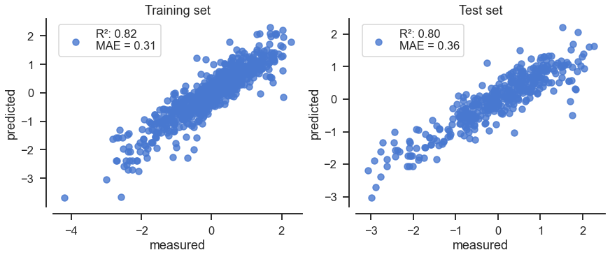
To assess the model, I will plot the predicted and measured solubilities:
[27]:
def plot_test_train_model(model, X_train, y_train, X_test, y_test):
    """Plot measured vs. predicted for test and train."""
    fig, (ax1, ax2) = plt.subplots(
        constrained_layout=True, ncols=2, figsize=(12, 5)
    )
    # Training:
    add_scatterplot(ax1, y_train, model.predict(X_train))
    ax1.set(xlabel="measured", ylabel="predicted", title="Training set")
    ax1.legend()
    # Testing:
    add_scatterplot(ax2, y_test, model.predict(X_test))
    ax2.set(xlabel="measured", ylabel="predicted", title="Test set")
    ax2.legend()
    sns.despine(fig=fig, offset=10)
[28]:
plot_test_train_model(model, X_train, y_train, X_test, y_test)

That looks promising (Note: the MAE is here calculated for the scaled data).
Let us compare with the measured solubilities and the ESOL predicted solubilities. For the comparison, I transform the output from the model back to solubilities:
[29]:
X = scale_x.transform(X_raw)
y_pred = model.predict(X)
model_predict = scale_y.inverse_transform(y_pred.reshape(-1, 1)).flatten()
models_table = {
    "Measured": measured,
    "ESOL": esol,
    "CatBoost": model_predict,
}
models_table = pd.DataFrame(models_table)
[30]:
fig, (ax1, ax2) = plt.subplots(
    constrained_layout=True, ncols=2, figsize=(12, 5)
)
ax2.scatter([], [])  # Just to cycle colors
for key in models_table:
    sns.kdeplot(
        data=models_table,
        x=key,
        ax=ax1,
        label=key,
        lw=5,
    )
    if key != "Measured":
        add_scatterplot(
            ax2, models_table["Measured"], models_table[key], model_name=key
        )

ax1.legend()
ax1.set(xlabel="Solubility", title="Distribution of solubilities")
ax2.set(
    xlabel="Measured solubility",
    ylabel="Predicted solubility",
    title="Measured vs. predicted",
)
ax2.legend()
sns.despine(fig=fig, offset=10)

The model seems to improve the over/underestimation in ESOL. But the new model uses many variables. Let us inspect it to see if we can simplify it.
Inspecting the model and creating a simplified model#
To simplify the model, I aim to create a linear model with few (say 4) features. To select these features I inspect their importance and shap values:
[31]:
feature_importance = model.get_feature_importance()
idx = np.argsort(feature_importance)
pos = np.arange(len(idx))

# Just show the 10 most important:
fig, ax = plt.subplots(constrained_layout=True, figsize=(8, 6))
ax.set_yticks(pos)
ax.set_yticklabels(variables[idx])
ax.barh(pos[-10:], feature_importance[idx[-10:]])
ax.set(xlabel="Feature importance")
sns.despine(fig=fig, offset=10)

[32]:
import shap

explainer = shap.Explainer(model, feature_names=variables)
shap_values = explainer(X)
[33]:
fig, ax = plt.subplots()
shap.summary_plot(
    shap_values,
    features=X,
    show=False,
    max_display=10,
)
cbar = fig.axes[-1]
cbar.set_aspect("auto")
fig.tight_layout()
cbar.set_box_aspect(25)
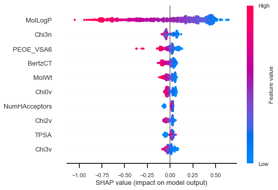
Here we see, for instance, that a higher MolLogP has a negative impact on solubility and that a lower molecular weight (MolWt) has a positive impact. This is probably what you could have guessed before making the model. Here is a closer inspection of the molecule with the highest solubility:
[34]:
shap.plots.waterfall(shap_values[idx_max])

and for the lowest solubility:
[35]:
shap.plots.waterfall(shap_values[idx_min])

We see here that MolLogP has a positive impact on the prediction for the molecule with highest solubility, and a negative impact for the molecule with the lowest solubility.
OK, so we have an idea of the most important variables. Let pick 4 simple ones (from the first plot of the feature importance) and make a linear model, for instance:
MolLogP(Wildman-Crippen LogP value.)MolWt(The molecular weight.)MinPartialCharge(Smallest Gasteiger partial charge.)NOCount(Number of Nitrogens and Oxygens.)
[36]:
variables2 = [
    "MolLogP",
    "MolWt",
    "MinPartialCharge",
    "NOCount",
]
[37]:
X_raw2 = rdkit_descriptors[variables2].to_numpy()

X_train2, X_test2, y_train2, y_test2, scale_x2, scale_y2 = split_and_scale(
    X_raw2, y_raw
)
[38]:
from sklearn.linear_model import Lasso
from sklearn.model_selection import GridSearchCV
[39]:
%%time
parameters = {
    "alpha": np.logspace(-3, 0, 20),
}
grid = GridSearchCV(
    Lasso(fit_intercept=False, max_iter=10000),
    parameters,
    cv=10,
)
grid.fit(X_train2, y_train2)
model2 = grid.best_estimator_
model2
CPU times: user 201 ms, sys: 3.51 ms, total: 204 ms
Wall time: 169 ms
[39]:
Lasso(alpha=0.00206913808111479, fit_intercept=False, max_iter=10000)In a Jupyter environment, please rerun this cell to show the HTML representation or trust the notebook.
On GitHub, the HTML representation is unable to render, please try loading this page with nbviewer.org.
Lasso(alpha=0.00206913808111479, fit_intercept=False, max_iter=10000)
[40]:
plot_test_train_model(model2, X_train2, y_train2, X_test2, y_test2)
The simplified model is:
[41]:
from IPython.display import display, Math

terms = [
    f"{i:.2g}×(\\text{{{var}}})" for i, var in zip(model2.coef_, variables2)
]
equation = "y =" + "".join(terms)
display(Math(equation))
This simplified model has a performance similar to the ESOL model.
Summary#
The CatBoost model for the solubility is pretty good with a coefficient of determination of 0.93 for the test set. And this was without tuning hyper-parameters.
The feature importances and shap values help understand the influence of the different features and based on these, a simplified model (with 4 variables) can be created that is performing similarly to the original ESOL model.